Michelle Thompson W5NYV and Matthew Wishek NB0X presented about the Role of Artificial Intelligence and Machine Learning (AI/ML) in Register Transfer Logic Design (RTL) Generation at a joint meeting of Open Source Digital Radio IEEE Local Group and the San Diego Chapter of the IEEE Information Theory Society. The meeting was held on 28 January 2025 and a recording can be found at https://youtu.be/8xDxeUxWTCc
AI/ML in RTL Design Generation Meeting Summary
In the meeting, Michelle and Matthew presented about the potential of artificial intelligence and machine learning in Electronic Design Automation (EDA) frameworks and the RTL design generation process. They identified core concepts from an open-source perspective and discussed the importance of reducing schedule, technical, and cost risks in the design process. Matthew highlighted the iterative nature of the design process and the need for early identification of design deficiencies and incorrect assumptions. He also suggested the use of AI agents to guide the high-level synthesis process, assist in design space exploration, and improve the performance of place and route.
Michelle discussed the potential of open-source EDA and recommendations from a European white paper, highlighting the challenges of limited access to EDA software and the workforce shortage. She mentioned the positive impact of open-source initiatives like the RISC-V processor and the Google Skywater Process Design Kit (PDK). The techincal recommendations included focusing more on multiple areas including analog and mixed-signal designs, interoperability and verification, and system-on-chip integration. She also emphasized the importance of proper licensing, funding, sustainability, and industry training for both open-source and AI/ML projects and highlighted the recommendation from Free and Open Source Silicon (FOSSi) Foundation for more conferences and events to better understand and filter the vast amount of information in the field.
Michelle discussed the use of large language models and automated writing of HDL for design IP. She shared her experience with ORI’s Remote Labs Matlab HDL Coder toolbox, which can produce high-quality, human-readable HDL code but requires a lengthy process and is not suitable for complex monolithic designs. She also mentioned the use of AI and ML in deep learning hardware models and their potential to inform the design process. Michelle also presented a survey of experts in the field, which showed a bias towards high-quality from proprietary tools and lower quality expectations from open source and AI/ML tools. Matthew then introduced a set of relevant papers he had found in his literature search, focusing on areas such as RTL generation, hardware verification, testbench generation, and formal verification. He emphasized the potential of these papers to inform and improve the design process.
Matthew presented about the role of of AI/ML in analog design, signal processing, and network planning. He suggested that AI tools can help with analog design, potentially enabling non-specialists to experiment and learn. He discussed the use of AI/ML in detecting convolutional codes, channel estimation, and radio map generation for network planning. There is significant overlap with information theory in these applications, particularly in tracking entropy levels in codes and signals. Michelle mentioned the potential for presentations on this topic at the Information Theory and Applications Conference 9-14 February 2025. Michelle also highlighted successful technology demonstrations by DARPA in 2019 showing improved spectrum efficiency using AI/ML models.
Daniel, Michelle, and Matthew discussed the pros and cons of using proprietary versus open-source Electronic Design Automation (EDA) tools. Michelle described the challenges of open-source projects, such as the lack of funding, limited market size, and difficulty in maintaining quality. Matthew shared his experience with open-source simulators, noting their limitations in terms of feature set parity and language coverage. Daniel suggested that open-source solutions might take longer to develop but could benefit from advancements in AI tools. Michelle and Matthew agreed that the EDA market is small, which contributes to the high cost of proprietary tools. The consensus from the participants was that while there are good open-source projects addressing AI/ML in RTL design generation, many of them may not yet be ready for complex designs.
Future Work for ORI AI/ML Team
It was resolved to pick one or more of the many tools and projects mentioned in the presentation, and give it a try. Reports about the first-hand experiences would then be shared in future IEEE meeting collaborations, to put the recommendations from FOSSi and the rubrics from Matthew into better context.
Open Research Institute is a non-profit dedicated to open source digital radio work. We do both technical and regulatory work. Our designs are intended for both space and terrestrial deployment. We’re all volunteer.
Membership is free. All work is published to the general public at no cost. Our work can be reviewed and designs downloaded at https://github.com/OpenResearchInstitute
We equally value ethical behavior and over-the-air demonstrations of innovative and relevant open source solutions. We offer remotely accessible lab benches for microwave band radio hardware and software development. We host meetups and events at least once a week. Members come from around the world.
Person 1: Hey, whatcha doing? Looks like something cool.
Person 2: Working on a Simulink model for an MSK model.
Person 1: Oh, that’s fun, how about I code up the modem in VHDL this weekend?
Person 2: Sounds great!
Famous last words, amirite? It has been many months – ahem 10 – since that pseudo conversation occurred. In that time there have been missteps, mistakes, and misery. We have come a long way, with internal digital and external analog loopback now working consistently, although unit to unit transmission isn’t quite there yet.
This is one way to do hardware development. Write some HDL code, simulate, and iterate. Once the simulation looks good, put it in an FPGA, test it, and iterate. You’ll get there eventually, but there will be some hair pulling and teeth gnashing along the way. But, it is worth the effort when you finally see it working, regardless (and because) of all the dumb mistakes made along the way.
There are many ways to approach a design problem, some better than others, and as with all things engineering, it’s a trade-off based on the overall design context. At opposing ends of the spectrum we have empirical and theoretical approaches. Empirical: build based on experience, try it, fix it, rinse and repeat. And, theoretical: build based on theory, try it, fix it, etc. Ultimately we must meet in the middle (and there is never getting away from the testing and iterating).
Starting from first principles always serves us well. One of the niggling points in the Minimum-Shift Keying (MSK) development has been selection of bit-widths for the signal processing chains.
Person 1 (yeah, that’s me): I’ll code it up this weekend. Let’s see, for the modulator we need data in, that’s 1-bit. The data gets encoded, still 1-bit. The data modulates a sine wave, hmmm, how many bits should that be? Well the DAC is 12-bits, so we should use a 2’s complement 12-bit number. That seems right.
Person 1: Now for the demodulator. The ADC outputs 12-bits, so a 2’s complement 12-bit number. That gets multiplied by a sine wave, let’s use a 2’s complement 12-bit number since we did that in the modulator. The multiply output is 24-bits, ok. Now we integrate that 24-bit number over a bit-period, hmmm, how many bits after the integration? No worries, let’s just make it 32-bits and keep on. But that is a lot of bits, let’s just scale the 32-bits down to 16-bits and keep going. Ah, the empirical approach, I’m getting so much done!
Person 1: Why isn’t this working? Oh, the 16-bit number is overflowing. I wish I could just make it 32-bits again, but that’s too many bits for the multiplier.
There is a better way! We can analyze the design from some starting point, such as, the number of input bits. From there we operate on those bits, adding, subtracting, multiplying, shifting, etc. And we know how each of those operations affects the bit widths, which allows us to choose appropriate bit-widths through the signal chain. Before we get there we need to take a quick look at fixed point math and related notation.
In our everyday base 10 math we have, essentially, infinite precision. One example is that irrational numbers can be expressed as fractions, and we can operate on those fractions and the infinite precision is maintained as long as we can keep the fractional representation. Often, though, we will need to use an approximation of the fraction to get an actual answer to a problem. One example is 1/3=0.33333… and we have to choose how many digits of 3 we need for the particular problem at hand. And, we know there is an error term when we use such an estimation (1/3=0.333+).
Base 2 math is largely the same, but hardware can’t use fractional representations, meaning that an irrational number will always be a finite representation. Also, we may be constrained in how many bits we can use to represent numbers. We need a way to notate these numbers.
Texas Instruments created Q-notation as a way to specify fixed-point numbers. The notation Qm.n is used to represent a signed 2’s complement number where m is the number of whole bits and n is the number of fractional bits. TI specifies m to not include the sign-bit, while ARM specifies m to include the sign bit. The table below shows examples of Q-notation using both TI and ARM variants.
Table 1. Q-Notation Examples
Total Bits
ARM Q Format
TI Q Format
Range
Resolution
8
Q3.5
Q2.5
-4.0 to +3.96875
2−5
16
Q4.12
Q3.12
-8.0 to +7.9997558594
2−12
24
Q8.16
Q7.16
-128.0 to +127.9999847412
2−16
32
Q8.24
Q7.24
-128.0 to +127.9999999404
2−24
8
UQ8.3
UQ8.3
0.0 to +255.875
2−3
10
Q1.10
Q10
-1.0 to +0.9990234375
2−10
The table below shows how bit widths are affected by various operations.
Table 2. Math operators affect on bit-widths
Operation
Input Numbers
Output
+/-
Qm.n +/- Qx.y
Qj.k where j = max(m,x)+1 and k = max(n,y)
*
Qm.n * Qx.y
Q(m+x).(n+y)
>>
Qm.n >> k
Qm.(n-k)
<<
Qm.n << j
Qm(n+j)
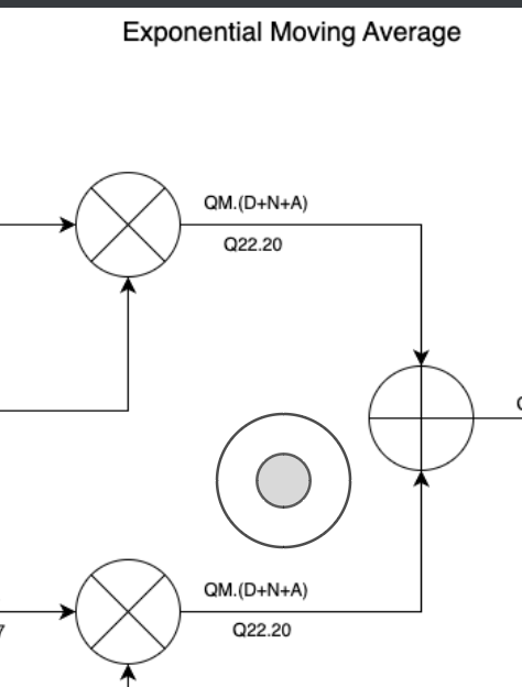
The diagram below shows an exponential moving average circuit with signal bit-widths notated as Qm.d. You can see the bit widths adjusted as we shift, multiply, add, etc. Since the output is an average of the input, it should have the same representation as the input (Qm.d). The lower representation (i.e. Q22.0 for the input) is an actual bit-width selection based on targeting the Zynq7010 and its 25×18 hardware multipliers. Some particular notes:
The Q22.0 input is specified by the surrounding system. It is left-shifted by 2-bits (Q22.2) to fully utilize the 25-bit multiplier input thus increasing the resolution.
The alpha input is specifically chosen to be Q17 to fully utilize the 18-bit multiplier input.
The bottom multiplier is in a feedback path, its output must match the upper multiplier output so that the binary points are aligned into the adder. To this end the adder output is truncated and rounded by 18-bits.
Figure 1. Exponential Moving Average Block Diagram
The adder output is truncated and rounded by 20-bits for the final output.
In summary Q-notation is a useful tool for understanding and specifying system bit-widths throughout the processing chain. It is especially useful to add Q-notation to the block diagram to help visualize the bit-widths. With this approach the optimal bit-widths should become apparent when taking into account system requirements. Doing this system analysis step before writing any code will save time and effort by reducing errors. The other benefit is that device resources are not over utilized, which may make the difference between fitting in an FPGA or not.
Additional reading and resources are available at these URLs:
A Python package for Fixed-point math is at fixedpoint 1.0.1 Package Documentation including explanations of Q-notation and how bit-widths are affected by arithmetic.
As the saying goes, mind your Ps and Qs.
Matthew Wishek, NB0X
Opulent Voice moves from real to complex modulation. Read on to find out more!
Real and Complex Signal Basics
The magic of radio is rooted in mathematics. Some of that math can be complicated or scary looking. We are going to break things down bit by bit, so that we can better understand what it means when we say that we are going to transmit a complex baseband signal.
Everything that we are going to talk about today is based on a single carrier real signal, even when we get to complex transmission. A single carrier real signal is where we take our data, a single-dimensional value that we want to communicate, and we multiply it by a carrier wave (a cosine wave) at a carrier frequency (fc). Let’s call the value we want to communciate “alpha”.
Because we are dealing with digital signals, the value that we are transmitting is held for a period of time, called T. The next period of time we send another constant value. And, so on. We are sending discrete values for a period of time T, one after another until we are all done sending data, and not continuous values over time.
Let’s say we are sending four different amplitudes to represent four different values. During each time period T we select one of these four amplitude values. We hold that value for the entire time period. These values can be thought of as single dimensional values. One value uniquely identifies the value we want to send. In this case, amplitude.
Sending one of four values at a time means we are sending two bits of data at a time.
alpha
bits
0
00
1
01
2
10
3
11
In order to send our value out over the air from transmitter to receiver, we multiply our alpha by our carrier frequency. The result is alpha*cos(2*pi*fc*t). Cosine is a function of time t. The 2*pi term converts radians per second to cycles per second, which is something that most of us find easier to deal with. When we multiply in the time domain, we cause a different mathematical thing to happen in the frequency domain. Multiplication is called convolution in the frequency domain. This mathematical process creates images, or copies, of our baseband signal in the frequency domain. One image will be located at fc and the other will be located at -fc.
Our real signal has a special characteristic. It’s symmetric. At the receiver, we multiply what we receive by that same cosine wave, cos(2*pi*fc*t). We multiply in the time domain, and we convolve in the frequency domain. This results in images at 2*fc, -2*fc, and most useful to us, we get two images at 0 Hz. We use a low-pass filter to get rid of the unwanted images at 2*fc and -2*fc, and by integrating over the time period T, we get a scaled version of the original value (alpha) that was sent. Amazing! We reversed the process and we got our original sent value.
So what’s all this complex signal stuff all about? Why mess with success? We have our single carrier signal and our four values. What more could we want?
Well, we want to be able to send more than a shave and a haircut number of bits!
If we want to send more bits in the same time period (and who doesn’t?) then we must use a bigger alphabet. Let’s double our throughput. We now pick from sixteen different amplitudes, sending the value we picked out for a period of time T as a single-carrier real signal. Now, each alpha value stands for four bits.
We have a minor problem. Sending out sixteen different voltage levels on a single carrier means that we have to be able to differentiate between finer and finer resolution at our receiver. Before, we only had to distinguish between four different levels. Now we have sixteen. This means we better have a really clear channel and a lot of transmit power. But, we don’t always have that. It’s expensive and a bit unreasonable. There is a better way.
We know we now want to send out (at least) one of sixteen values, not just one of four. If we turn our one-dimensional problem into a two-dimensional problem, and assign a real single carrier signal to, say, the vertical dimension, and then a second real single carrier signal to the horizontal dimension, then we are now enjoying the outer limits of digital signal processing. The vertical handles four levels. The horizontal handles four levels.
We still have the same time period T. We just have a two-dimensional coordinate system instead of a one-dimensional coordinate system.
alpha
bits
alpha
bits
0
0000
8
1000
1
0001
9
1001
2
0010
10
1010
3
0011
11
1011
4
0100
12
1100
5
0101
13
1101
6
0110
14
1110
7
0111
15
1111
But how can we send two real signals over the air, at the same time? We can’t just add them together, can we? They will step on each other and we’ll get a noisy mess at the receiver. Math saves us! We can actually add these two signals together, send them as a sum, and then extract each dimension back out. But, only if we prepare them properly. And here is how that is done.
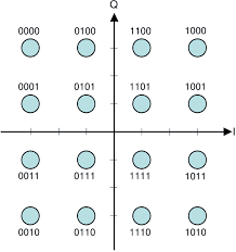
Look at the two-dimensional diagram of 16QAM. The vertical axis is labeled Q, and the horizontal axis is labeled I. When we want to indicate the vertical dimension of our value (pick any one of them), then we take that vertical dimension (say, -1 for 1111) and we multiply it by sin(2*pi*fc*t). We now have our Q signal. Now we need the horizontal location of 1111. That would be +1 on the I axis. We multiply this value, giving the horizontal dimension, by cos(2*pi*fc*t). We now have our I signal. Q axis value was multiplied by sine. I axis value was multiplied by cosine. These signals are played for the duration of the sample period. Both of them happen at the same time to give a coordinate pair for a particular alpha.
We add the I and Q signals together and transmit them. We are sending (I axis value) * cos(2*pi*fc*t) + (Q axis value) * sin(2*pi*fc*t).
At the receiver, we take what we get and we split the signal. We now have two copies of what we received. We multiply one copy by cos(2*pi*fc*t). We multiply the other by sin(2*pi*fc*t). We integrate over our time period T. This is important because it lets us take advantage of several trig identities.
First, let’s multiply and distribute our cos(2*pi*tfc*t) across the summed signals we received. We multiply:
Aha! We can convert that cos2() term to something we can use. Use the half angle identity, square each side, and double all the angle measurements (easy, right?). After this cleverness, this is what we have.
cos2(2*pi*fc*t) = 1/2*[1 + cos(2*pi*2fc*t)]
So now we have
(I axis value) * 1/2*[1 + cos(2*pi*2fc*t)]
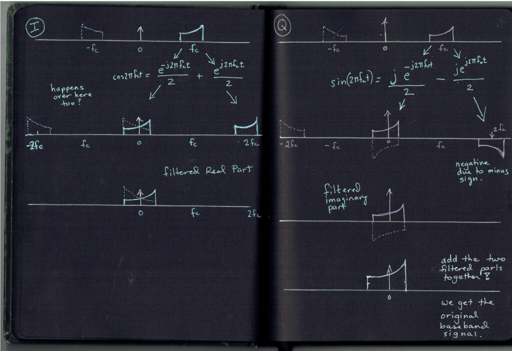
See that 2fc term in there? Check out the notebook drawing for our signal in the frequency domain. It’s at 2fc. Q signal is on the right-hand half of the drawing.
Let’s rearrange things.
(I axis value/2) + [(I axis value/2) * cos(2*pi*2fc*t)]
Remember we are integrating over time at the receiver. We have one of the two terms rewritten in a useful way. What happens when we integrate a cosine signal from 0 to T? That value happens to be zero! This leaves just the integration of (I axis value/2)!
The result at the receiver for the multiplication and integration of the first copy of the received signal is (I axis value)*(T/2). We know T, we know what the number 2 is, so we know the I axis dimension value.
But wait! We forgot something. We only did the first part.
We recovered I axis value from the term before the plus sign. But what about the term after the plus sign?
(Q axis value) * sin(2*pi*fc*t)*cos(2*pi*fc*t)
Uh oh we didn’t get away from summing the I and Q together after all…
Trig saves us here too. When we integrate sin(2*pi*fc*t)*cos(2*pi*fc*t) from 0 to period T, it happens to be zero. The entire Q axis value term drops out. Does the same technique work for the copy of the received signal that we multiply by sin(2*pi*fc*t)?
You bet it does! First, let’s multiply and distribute our sin(2*pi*tfc*t) across the second copy of the summed I and Q signals we received. We multiply:
Now that we know that integrating cos(2*pi*fc*t)sin(2*pi*fc*t) from 0 to T is zero, we can drop out the I axis value term. That’s good because we already have it from multiplying our received summed signal by cos(2*pi*fc*t) and doing trigonomtry tricks.
We are left with
(Q axis value) * sin(2*pi*fc*t)*sin(2*pi*fc*t)
And we rewrite it
(Q axis value) * sin2(2*pi*fc*t)
And use the half angle trig identity, square each side, and then double all angle measurements.
Hey, guess who goes to zero again? That’s right, cosine integrated from 0 to T is zero. We are left with a constant term that integrates out to (Q axis value) * (T/2)
So when we multiply the summed signal that we received by cosine, we get I axis value. When we multiply the summed signal that we received by sine, we get Q axis value.
I and Q give us the coordinates on the 16 QAM chart. As long as we are in sync with our transmitter (a whole other story) and as long as our map of which point stands for which label (read your documentation!) is the same as at the transmitter, then we have successfully received what was sent using a technique called quadrature mixing.
Moving from a single carrier real signal to a “complex” signal, where two real signals are sent at the same time using math to separate them at the receiver, gives us advantages with respect to sending more bits without having to send more levels. Our two signals are each handling four levels, but using the results in a two-dimensional grid gives us more bits per unit time without having to change our performance expectations. Sending sixteen different levels is harder than sending four. So, we send four twice and use some mathematical cleverness.
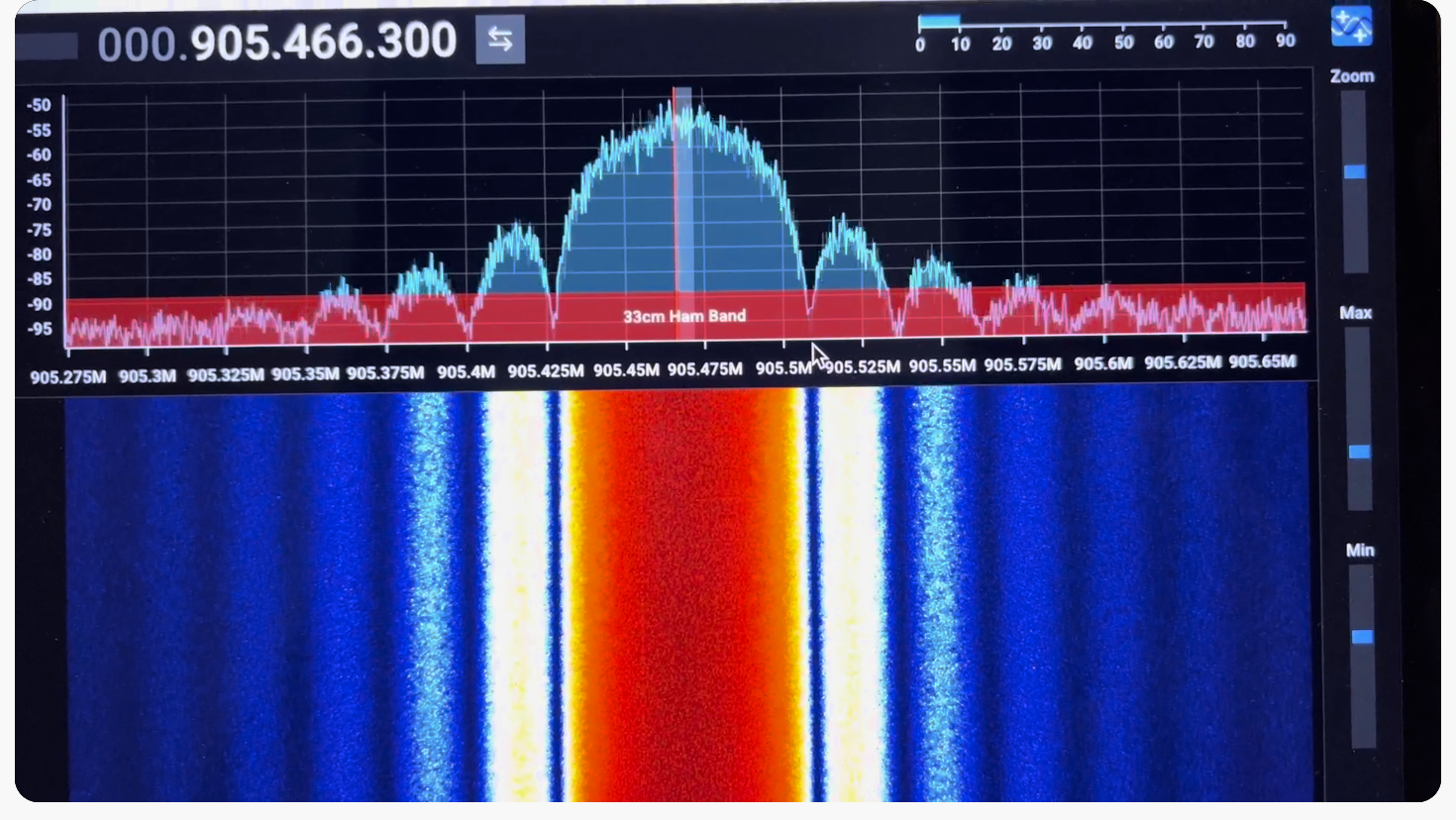
However, doing this complex modulation scheme gives us yet another advantage. Because of the math we just did, we eliminate an entire image when compared to a single carrier real signal. We have a less difficult time with filters because we no longer create a second image. Below (next page) are some diagrams of how this happens.
A third advantage of I and Q modulation is that it doesn’t just do things like 16QAM. Using an I and a Q, and a fast enough sample period T, means you can send any type of modulation or waveform. Now that’s some power!
This technique does require some signal processing at the receiver. But, this type of signal handling is at the heart of every software defined radio. And, now you know how it’s done, and the reasons why Opulent Voice is now using complex modulation in the PLUTO SDR implementation.
-Michelle Thompson W5NYV
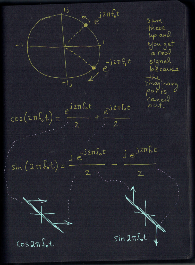
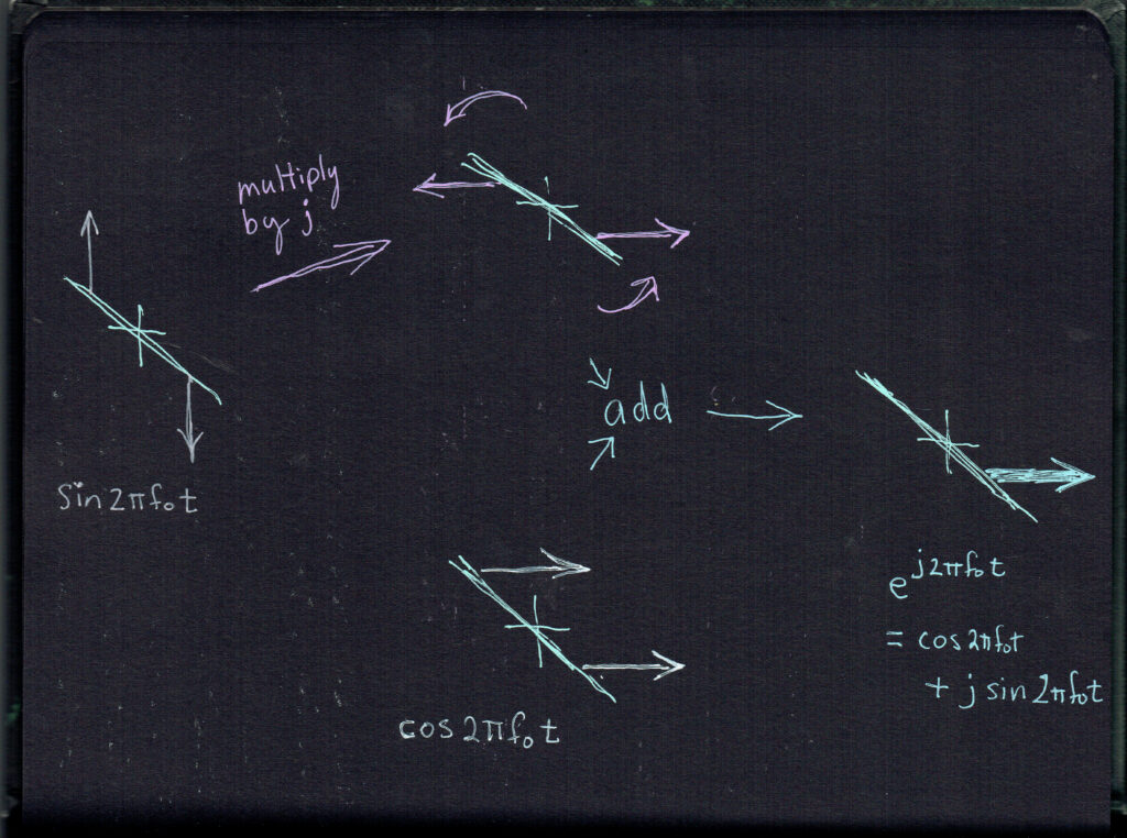
(Below are two more pages from our lab notebook, showing a few more visual representations. Don’t let the exponential functions worry you – “e” is a more compact way of representing the sine and cosine functions. In our notebook we show how sine and cosine can add to a single image. We can do this because sine and cosine are independent in a special way. This quality of “orthogonality” is used in all digital radios.)
Adding a Preamble to Opulent Voice
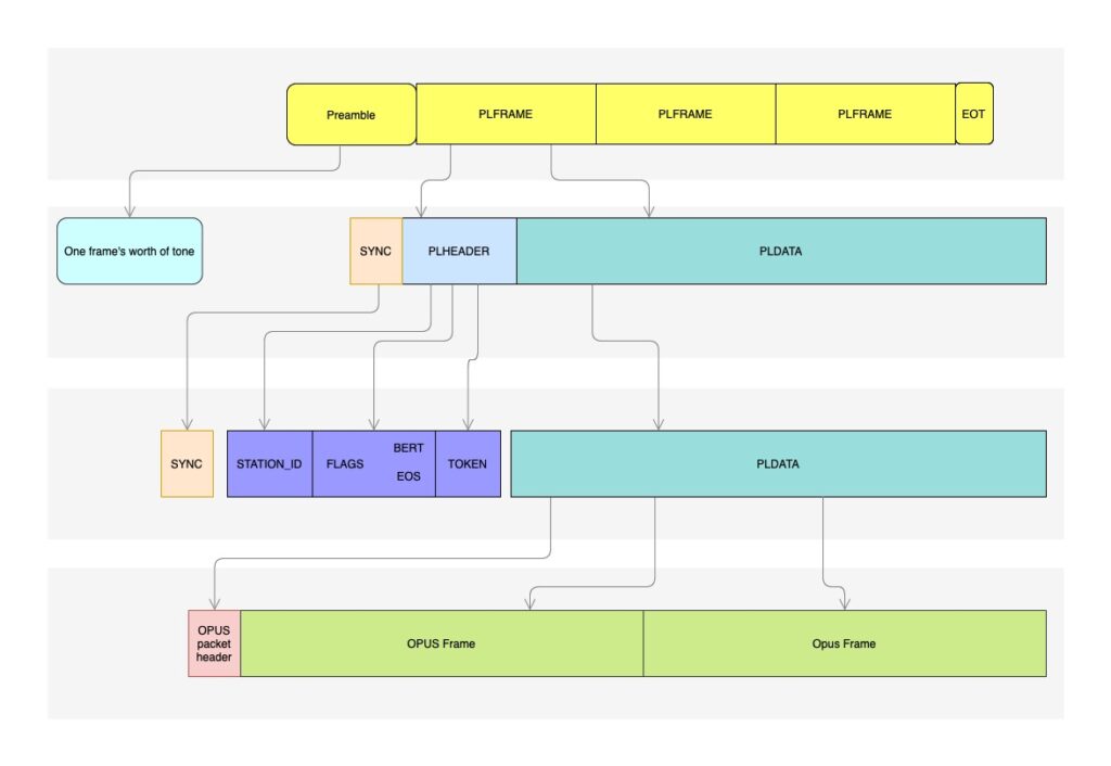
Looking at the Opulent Voice protocol overview diagram below, we can see that each transmission begins with a preamble. This section of the transmission contains no data, but is extremely helpful in receiving our digital signal.
The preamble is like a lighthouse for the receiver, revealing a shoreline through the fog and darkness of interference and noise. While we may not need the entire 40 milliseconds of preamble signal to acquire phase and frequency, so that we are “on board” for the rest of the transmission, keeping the preamble at the length of a frame simplifies the protocol.
There is a similar end of transmission (EOT) frame, so that the receiver knows for sure that the transmitted signal has ended, and has not simply been lost. This will reduce the uncertainty at the receiver, and allow it to return to searching for new signals faster and more efficiently.
For minimum shift keying, the modulation of Opulent Voice, a recommended preamble data stream in binary is 1100 repeating. In other words, we’d get a frame’s worth of 11001100110011001100… at 54.2 kilobits per second for 40 milliseconds.
After the preamble is sent, data frames are sent. Note that there is a synchronization segment at the beginning of each frame. This keeps the receiver from drifting and improves reliability.
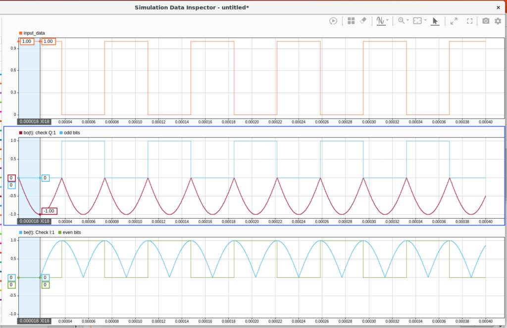
Constructing the Preamble in Simulink and in HDL
Below is the Simulink model output viewer showing the 1100 repeating pattern mathematical construction, followed by the planned update for the hardware description language (HDL) code updates. The target for HDL firmware is the PLUTO SDR. -Opulent Voice Team
“Take This Job”
Interested in Open Source software and hardware? Not sure how to get started? Here’s some places to begin at Open Research Institute. If you would like to take on one of these tasks, please write hello@openresearch.institute and let us know which one. We will onboard you onto the team and get you started.
Opulent Voice:
Add a carrier sync lock detector in VHDL. After the receiver has successfully synchronized to the carrier, a signal needs to be presented to the application layer that indicates success. Work output is tested VHDL code.
Bit Error Rate (BER) waterfall curves for Additive White Gaussian Noise (AWGN) channel.
Bit Error Rate (BER) waterfall curves for Doppler shift.
Bit Error Rate (BER) waterfall curves for other channels and impairments.
Review Proportional-Integral Gain design document and provide feedback for improvement.
Generate and write a pull request to include a Numerically Controlled Oscillator (NCO) design document for the repository located at https://github.com/OpenResearchInstitute/nco.
Generate and write a pull request to include a Pseudo Random Binary Sequence (PRBS) design document for the repository located at https://github.com/OpenResearchInstitute/prbs.
Generate and write a pull request to include a Minimum Shift Keying (MSK) Demodulator design document for the repository located at https://github.com/OpenResearchInstitute/msk_demodulator
Generate and write a pull request to include a Minimum Shift Keying (MSK) Modulator design document for the repository located at https://github.com/OpenResearchInstitute/msk_modulator
Evaluate loop stability with unscrambled data sequences of zeros or ones.
Determine and implement Eb/N0/SNR/EVM measurement. Work product is tested VHDL code.
Review implementation of Tx I/Q outputs to support mirror image cancellation at RF.
Haifuraiya:
HTML5 radio interface requirements, specifications, and prototype. This is the user interface for the satellite downlink, which is DVB-S2/X and contains all of the uplink Opulent Voice channel data. Using HTML5 allows any device with a browser and enough processor to provide a useful user interface. What should that interface look like? What functions should be prioritized and provided? A paper and/or slide presentation would be the work product of this project.
Default digital downlink requirements and specifications. This specifies what is transmitted on the downlink when no user data is present. Think of this as a modern test pattern, to help operators set up their stations quickly and efficiently. The data might rotate through all the modulation and coding, transmititng a short loop of known data. This would allow a receiver to calibrate their receiver performance against the modulation and coding signal to noise ratio (SNR) slope. A paper and/or slide presentation would be the work product of this project.
The Inner Circle Sphere of Activity
January 6, 2025 – All labs re-opened. Happy New Year!
January 13, 2025 – ORI presented to Deep Space Exploration Society about our history and projects line-up.
January 18, 2025 – San Diego Section of IEEE Annual Awards Banquet. ORI volunteers supported this event as a media and program sponsor. ORI was represented by five members.
January 23-26, 2025 – IEEE Annual Meeting for Region 6 and Region 4, ORI was represented by three members.
January 28, 2025 – Co-hosted the IEEE Talk “AI/ML Role in RTL Design Generation” with the Information Theory Society and the Open Source Digital Radio San Diego Section Local Group.
February 18, 2025 – San Diego County Engineering Council Annual Awards Banquet. ORI will be part of the IEEE Table display in the organizational fair held on site before dinner. ORI will be represented by at least one member.
Thank you to all who support our work! We certainly couldn’t do it without you.