The Who What When Where Why
Open Research Institute is a non-profit dedicated to open source digital radio work on the amateur bands. We do both technical and regulatory work. Our designs are intended for both space and terrestrial deployment. We’re all volunteer and we work to use and protect the amateur radio bands.
Subscribe to this newsletter here: http://eepurl.com/h_hYzL
You can get involved in our work by visiting https://openresearch.institute/getting-started
Membership is free. All work is published to the general public at no cost. Our work can be reviewed and designs downloaded at https://github.com/OpenResearchInstitute
We equally value ethical behavior and over-the-air demonstrations of innovative and relevant open source solutions. We offer remotely accessible lab benches for microwave band radio hardware and software development. We host meetups and events at least once a week. Members come from around the world.
This month’s puzzle update is a VHDL test bench for the August “bug report”.
Can you find the root cause using the test bench? Solution in next month’s issue.
Table of Contents
VHDL Test Bench Hint for August Puzzle
FutureGEO Workshop Memo
TX IIO Timeline Implementation for Opulent Voice
Finding Optimal Sync Words for Digital Voice Protocols
A Day at Dwingeloo
Comment and Critique on “Real and Complex Signal Basics”
Mode Dynamic Transponder Analysis and Proposal for AMSAT-UK
August Issue: VHDL Puzzle Hint
Here is a comprehensive testbench that systematically exposes the problem through various test scenarios. What could possibly be causing the problem? You can run this to see the intermittent failures and gather evidence pointing toward error starvation.
Link to .vhd file here:
https://github.com/OpenResearchInstitute/documents/blob/master/Papers_Articles_Presentations/Articles_and_Announcements/error_starvation_hint.vhd
FutureGEO Workshop Memo
See https://gitlab.com/amsat-dl/futuregeo for more information and the most recent version of this memo.
Presentations
A FutureGEO Project Workshop was held 19 September 2025. The event was organized by AMSAT-DL with sponsorship and support from the European Space Agency (ESA). The workshop was immediately before AMSAT-DL’s Symposium and Membership Meeting, which was 20-21 September 2025.
Peter Gülzow, President and Member of the Board of Directors of AMSAT-DL, opened the workshop, expressing hope for good results.
Peter described the timeline and progression of payloads from SYNCART to QO-100 to FutureGEO. The QO-100 timeline from 2012 to 2018 was explained. QO-100 had some iteration along the way. In the end, AMSAT-DL provided the complete specifications for the custom hardware, which were implemented by Es’hailSat and MELCO. Thus, QO-100 was by no means a “detuned commercial transponder,” as ome describe, but was largely composed of tailor-made custom function blocks and circuits. Some commercial off-the-shelf parts were used, in particular both traveling wave tube (TWT) amplifiers used in the NB and WB. These are in fact the “backup” TWT’s for the commercial transponders and can be swapped if neccessary.
Volunteer amateurs were unfortunately not directy involved in the building of the satellite. The fact that AMSAT-DL did not build any flight hardware itself was solely due to insurance and liability reasons. With a project volume of US$300–400 million including launch, no insurance company was willing to provide affordable coverage, and in the worst case the personal liability of the AMSAT-DL board members would have been at stake. In the end, it was a win-win situation for AMSAT, because MELCO not only built redundant modules, but also bears full responsibility and guarantees the planned service life of the satellite to the client.
Nevertheless, AMSAT-DL was still deeply involved in Hardware Building blocks: the team defined the requirements and specifications, carried out requirements reviews, the Critical Design Review, final reviews, and participated in quality assurance together with MELCO and Es’hailSat. In addition, AMSAT-DL built the ground station equipment for the spacecraft control center (SCC) consisting of two racks including the beacons, DATV, LEILA, and monitoring. Similar ground stations were also set up in Bochum and at the QARS headquarters.
Peter also explained that the entity that builds the host payload makes a tremendous difference in what the payload looks like, how much power is available, and what policies the hosted payload will be operated under. Es’hail-2 was build by MELCO in Japan, and their decisions set the possibilities and the limitations for the QO-100 hosted payload. We may face similar conditions with a futureGEO.
For FutureGEO, multiple designs are expected, covering a range of options and systems design theories.
The 47 degree West footprint shown in slides and online is “a wish”. No launch or orbital slot has yet been chosen.
Presentations continued with Frank Zeppenfeldt PD0AP, from the European Space Agency Satellite Communications Group.
Frank explained that there is interest from ESA on a follow-up to QO-100. This lead to the formal solicitation as described in ESA ARTES Future Preparation 1A.126. The FutureGEO outreach and community building process started in 2023. Frank admitted that the communications from ESA have not been as frequent or consistent as desired over the past 18 months. Frank highlighted this workshop as demonstrating an improved FutureGEO community and consensus building state of activity.
AMSAT-DL will help evaluate proposals and is responsible for completing tasks outlined in the ARTES solicitation.
GEO opportunities are hard to get. It’s is hard to get a slot. As a way to move the process forward, ESA has indicated that a budget of up to 200,000 € could be allocated in a future phase of ARTES, if the current feasibility study leads to continuation. This would also include funding or building prototypes. However, for the present workshop, only a much smaller preparatory amount was provided, covering infrastructure and moderation costs.
Amateur built payloads are unlikely to fly. But, we must have a number of ideas documented and prototyped so that we are ready to fly something that we want as a community. For example, 18 months ago there was a missed opportunity in the 71-81 GHz band. Ideas need to be developed, and then there will be financing.
Peter then explained about attempts to get EU launches. This was very difficult. Peter said that not everyone was welcoming of an amateur payload, and that there were complicated and challenging discussions.
Peter reviewed the objective and scope of the ARTES Statement of Work, and then outlined the progress on Tasks 1 through 3.
Task 1 was to identify parties and stakeholders in amateur radio that should be reached out to, and to provide basic storage for data from consultations. Also, to provide background and briefing material about FutureGEO. AMSAT-DL set up a GitLab instance for FutureGEO documents and has provided a chat server for participants.
Task 2 work products are an actively maintained discussion forum on the website, documentation of lessons learned with QO-100, documentation describing requirements formulated by amateur community, documentation describing and analyzing the initial payload proposals from the amateur community, including synergies with other amateur initiatives, and an actively updated stakeholder’s database. These parts of the task fall to AMSAT-DL. ESA support in this task will be providing additional contacts of individuals and industry active in the amateur satellite world, initial publicity using ESA’s communication channels, and technical support in assessing payload and ground segment options.
Task 3 is to analyze and consolidate 3-4 big/small HEO/GEO designs. The designs need to be interesting for a broad community and also address the need for developing younger engineers. Technologies considered may include software defined radio (SDR), communication theory, field programmable gate arrays (FPGA) and more. A report on the workshop discussions and conclusions is expected along with a report describing the consolidated satellite amateur missions.
Task 1 has been satisfied. This FutureGEO workshop was part of the process of completing Tasks 2 and 3.
Workshop Participants
Thomas Telkamp PA8Z Amateur Operator
Danny Orban ON4AOD Amateur Operator
Bill Slade (with Danny) Amateur Operator
Nicole Sehrig Bochum Observatory
Frank Zeppenfeldt PD0AP ESA
Ken Easton Open Research Institute
Michelle Thompson W5NYV Open Research Institute
Schyler Erle N0GIS ARDC
Brian Jacobs ZS6YZ South African Radio League
Hans van de Groenendaal ZS6AKV South African Radio League
Hennie Rheeder ZS6ALN South African Radio League
Peter Gülzow DB2OS AMSAT-DL
Thilo Elsner DJ5YM AMSAT-DL
Matthias Bopp DD1US AMSAT-DL
Félix Páez EA4GQS AMSAT-EA
Eduardo Alonso EA3GHS AMSAT-EA
Jacobo Diez AMSAT-EA
Christophe Mercier F1DTM, AMSAT-F
Nicolas Nolhier F5MDY AMSAT-F
Thomas Boutéraon F4IWP AMSAT-F
Michael Lipp HB9WDF AMSAT-HB
Martin Klaper HB9ARK AMSAT-HB
Graham Shirville G3VZV AMSAT-UK
David Bowman G0MRF AMSAT-UK
Andrew Glasbrenner K04MA AMSAT-USA
With audio-visual and logistics support from Jens Schoon DH6BB.
With moderation from Joachim Hecker, a highly-regarded science journalist and electrical engineer.
Brainstorming Session
Workshop participants then focused on answering questions in a moderated session about the satellite system design of a future amateur radio GEO spacecraft. Specific questions were posed at four stations. Workshop participants divided into four groups. Each group spent 20 minutes at each station. All groups visited each station, in turn. The content generated by the participants at the four stations was then assembled on boards. Participants clustered the responses into sensical categories. Then, all participants weighted the clusters in importance with stickers.
Board 1: Mission Services & Overall Architecture
“Your idea for the mission with regards to services offered and overall architecture.”
From on-site discussions:
Multiple antennas with beamforming.
Downlink (analog) all antennas? Beamform on the ground.
Physics experiment: measure temp, radiation, etc. Magnetometer.
Downlink in beacon.
For schools.
Something like Astro Pi, coding in space (put data in beacon).
Beacons are very important for reference for microwave. Beacons are good! 24GHz and higher, 10 GHz too.
GEO-LEO multi-orbit communications. In the drawing, communications from LEO to GEO and then from GEO to ground are indicated with arrows.
Doppler and ranging experiments.
Bent pipe and regenerative capability.
Store and forward capability?
Sensor fusion from earth observation, cameras, and data collection.
Multiple bands in and out, VHF to 122 GHz or above.
Inter-satellite links: GEO to GEO, GEO to MEO, GEO to LEO
Education: Still images of Earth, data sent twice in 2-10 minute period. High resolution?
Propagation: greater than or equal to 24 GHz.
Handheld very low data rate text service.
Asymmetric low data rate uplink, traditional downlink.
“Aggregate and broadcast”.
Cannot be blocked by local authority.
Use Adaptive Coding and Modulation (ACM) to serve many sizes of stations. Measure SNR, then assign codes and modulations.
Flexible band plan, do not fix entire band, leave room for experimentation.
From online whiteboard:
One sticky note was unreadable in the photograph.
Educational easy experiments requiring receive only equipment.
Same frequency bands as QO-100 to re-use the equipment.
Have a wideband camera as part of the beacon.
Maybe allow nonlinear modulation schemes.
Keep in mind “Straight to Graveyard” as an orbit option. Look not just for GEO but also MEO or “above GEO” drift orbit.
Look at lower frequency bands (VHF, UHF, L-band).
Make the community more digital.
We should have a linear bent-pipe transponder.
Enable Echolink type operations.
For emergency communications it would be useful to be able to pass text-based messages including pictures. Having more bandwidth helps for faster speeds.
We need telemetry, especially for working with students.
Power limitation?
Clustered topics:
Beacons
Coding (like Astro Pi)
Intersatellite links
Telemetry/Sensors
Text and image facilities for emergencies
Near-GEO options for orbits
Adaptive coding and modulation
Bands: transmit 5 GHz 24 GHz and receive 10 GHz 24 GHz 47 GHz 76 GHz 142 GHz
Ranging experiments
Bent pipe or regenerative (including mode changes input to output)
Board 2: Payload & Antenna Subsystem Platform
“Your idea for the payload and antenna subsystem, and their platform accommodation requirements.”
From on site discussions:
Phased Arrays:
Simple, fixed, e.g. horn array
Electronically steerable
Switchable
User base:
Large user base at launch with 2.4 GHz uplink 10 GHz downlink.
Good user base at launch with experiments.
Use the frame of the solar cells for HF receive.
Distributed power amplifiers on transmit antennas.
Array of Vivaldi antennas allows multiple frequencies with same array.
Camera at Earth “still” 1 image every 2 to 5 minutes. Camera at satellite for “selfie sat” images. AMSAT-UK coll 2012?
5 GHz uplink and 10 GHz downlink at the same time as 24 GHz uplink and 10 GHz downlink. 76 GHz 47 GHz beacon or switched drive from FPGA core (transponder).
Non-GEO attitude control? GEO 17 degree beamwidth.
ISAC integrated sensing and communications. For example, 24 GHz communications gives free environmental and weather information.
Keep in mind different accommodation models/opportunities. 16U, almost-GEO, MEO, very small GEO.
Optical beacon laser LED.
PSK telemetry.
Spot beam global USA + EU?
Uplink 10 GHz
Downlink 24 GHz, 47 GHz, 76 GHz
132 GHz and 142 GHz?
From online whiteboard:
If we need spotbeams especially at the higher frequencies we should have multiple and/or be flexible.
24 GHz uplink meanwhile is no more than expensive (homebuilt) transverter 2W, 3dB noise figure, approximately 400 Euros, ICOM is meanwhile supporting also 10 GHz and 24 GHz.
Beacons for synchronizing
Cameras: maybe one covering the Earth and one pointing to the stars (for education). Attitude calculation as a star tracker. Space weather on payload. Radiation dose or SEU?
On a GEO satellite we should not only have 12 cm band but for instance also the 6 cm band (WiFi) close by makes the parts cheap. For example, 90 watt for about 400 Euros.
We should have as back at AO40 we should have a matrix. For example, multiple uplink bands at the same time combined in one downlink.
Maybe get back to ZRO type tests.
Inter satellite link would be nice.
Higher frequency bands: use them or lose them.
Linking via ground stations makes sense for Africa being probably in the middle of GEO footprints.
One note was unreadable in the photo, but it starts out “beacon on the higher frequency bands would be interesting as a reference signal for people”
Clustered topics:
Phased arrays.
Large user base at launch from 2.4 GHz uplink and 10 GHz downlink. Good user base at launch from experiments.
Use frame of the solar cells for HF receive.
Keep in mind different accommodation models/opportunities. 16U, almost-GEO, MEO, very small GEO.
Camera for education
Education at lower level such as middle school (12-14 years old).
ISAC: Integrated sensing and communications, for example 24 GHz communications gives free environmental and weather information.
Transponders and frequencies.
Board 3: Ground Segment Operations & Control
“Your idea for the ground segment for operations and control of the payload, and the ground segment for the user traffic.”
From on-site discussions:
For hosted payloads, you have less control. For payloads without propulsion, there is less to control. Payloads with propulsion you have to concern yourself with control of the radios and the station position and disposal. There is a balance between being free to do what you want with the spacecraft and the ownership of control operations. This is a keen challenge. Someone has to own the control operations.
If you are non-GEO, then 3 or more command stations are required. Payload modes are on/off, limited by logic to prevent exceeding power budgets. Control ground station receives data (for example, images) and sends them to a web server for global access. This expands interest.
GEO operations may need fewer control operators. HEO (constellation or single) may need more.
Redundancy: multiple stations with the same capabilities.
Clock: stable and traceable (logging). For example, multi band GPSDO with measurement or White Rabbit to a pi maser?
Distribute clock over transponder and/or lock transponder to clock.
Open SDR concept, that the user can also use:
Maybe a Web SDR uplink
Scalable
Remote testing mode for users
Payload clock synchronized via uplink – on board clock disciplined to uplink beacon or GPS. Payload telemetry openly visible to users. Encryption of payload commands?
From online whiteboard:
Allow also an APRS type uplink for tracking, telemetry, maybe pictures, maybe hand-held text based two-way communications, etc. Which suggests low-gain omni-directional antennas.
Ground control for a GEO especially with respect to attitude will most likely be run 24/7 and thus hard for radio amateurs.
If we are using a GEO hosted payload then ground control of the satellite would be provided by the commercial operator.
If we want to have full control on the the payload such as the beacons: on QO-100 on the wide-band transponder we are limited as the uplink is from the commercial provider.
We should have some transponders with easy access (low requirements on the user ground segment) but it is ok to have higher demands on this on some others (like the higher GHz bands).
We will need multi band feeds for parabolic dishes.
Clustered Topics:
We want telemetry!
We should have some transponders with easy access (low requirements on the user ground segment) but it is ok to have higher demands on this on some others (like the higher GHz bands).
We will need multi band feeds for parabolic dishes.
Ownership and planning of payload control.
Redundancy: multiple stations with the same capabilities.
Clock: stable and traceable (logging). For example, multi band GPSDO with measurement or White Rabbit to a pi maser?
Distribute clock over transponder and/or lock transponder to clock.
Open SDR concept, that the user can also use:
Maybe a Web SDR uplink
Scalable
Remote testing mode for users
Board 4: User Segment
“Your idea for the user segment.”
From on-site discussions:
Entry-level phased array.
Look at usage patterns of QO-100 for what we should learn or do.
Capability to upload TLM to a central database. The user segment should allow us to start teaching things like OFDM, OTFS, etc.
Easy access to parts at 2.4 GHz, 5 GHz, 10 GHz, 24 GHz.
Broadband RX (HF, VHF, UHF) for experiments
LEO satellite relay service VHF/UHF
Single users: existing equipment makes it easy to get started. Low complexity. Linear.
Multiple access:
Code Division Multiple Access (CDMA), spread spectrum, Software Defined Radio + Personal Computer etc.
Orthogonal Frequency Division Multiplex (OFDM), with narrow digital channels.
Cost per user
Experimental millimeter wave
Something simple, linked to a smartphone, “Amateur device to device (D2D)” or beacon receive.
School-level user station in other words, something larger.
Entry-level off the shelf commercial transceivers.
Advanced uses publish complex open source SDR setups.
Extreme low power access: large antenna on satellite? ISM band? (Educational and school access)? “IoT” demodulator service
A fully digital regenerating multiplexed spacecraft: Frequency division multiple access uplink to a multi-rate polyphase receiver bank. If you cannot hear yourself in the downlink, then you are not assigned a channel. Downlink is single carrier (DVB-S2).
Mixing weather stations and uplink (like weather APRS).
Dual band feeds exist for 5/10 GHz and 10/24 GHz. We are primary on 47 GHz. Why not a 47/47 GHz system.
Keep costs down as much as possible.
From online whiteboard:
Linear transponder for analog voice most important but we should also allow digital modes for voice and data in reserved segments of the transponder.
Multiple uplinks combined in a joint downlink (as AO13 and AO40).
Experimental days.
Tuning aid for single sideband (SSB) audio.
Segment to facilitate echolink type operation using satellite in place of internet.
Allow low-power portable operations.
Allow experimental operations. For example, on very high frequencies.
Store and forward voice QSOs using a ground-based repeater and frequencies as MAILBOX (codec2 or clear voice + CTSS).
A codec2 at 700 bps/FSK could permit to reuse UHF radios using the microphone input and a laptop. We are exploring this using LEOs.
Depending on the available power we may want to allow non-linear modulation schemes.
We should support emergency operations.
Depending on the platform, we may want to rotate operational modes.
Clustered topics:
Simple (ready made) stations: off the shelf designs and 2.4 GHz 5.0 GHz 10 GHz 24 GHz 47 GHz
Sandbox for experiments and testing new modulations and operations. Just have to meet spectral requirements.
Workshop Retrospective:
A workshop retrospective round-table was held. QO-100 experiences were shared, with participants emphasizing the realized potential for sparking interest in both microwave theory and practice.
The satellite enabled smaller stations and smaller antennas. It is unfortunate that people building it were limited in speaking about the satellite performance due to non-disclosure agreements. QO-100 has enabled significant open source digital radio components, such as open source DVB-S2 encoders that are now in wide use. Educational outreach and low barriers to entry are very important. $2000 Euro stations are too expensive. The opportunity for individuals to learn about microwave design, beacons, and weather effects is a widely appreciated educational success. 10 GHz at first seemed “impossible” but now it’s “achievable”. QO-100 had a clear effect on the number of PLUTO SDRs ordered from Analog Devices, with the company expressing curiosity about who was ordering all these radios. GPSDO technology cost and complexity of integration has come down over time. Over time, we have seen continuous improvements in Doppler and timing accuracy. Building it vs. Buying it is a core question moving forward. A high level of technical skills are required in order to make successful modern spacecraft. Operators clearly benefited from QO-100, but we missed out on being able to build the hardware. Builder skills were not advanced as much due to the way things worked out. “What a shame we didn’t build it”. No telemetry on QO-100 is a loss. Design cycle was too short to get telemetry in the payload, and there were privacy concerns as well. Building QO-100 was an expensive and long process. Mitsubishi took this workload from us. Moving forward, we should strive to show people that they have agency over the communications equipment that they use. We are living in a time where people take communications for granted. There is great potential for returning a feeling of ownership to ordinary citizens, when it comes to being able to communicate on the amateur bands.
High-level Schedule and Goals:
Documentation of the workshop and “Lessons Learned from QO-100” will be done starting now through the end of 2025. Prototypes are expected to be demonstrated in 2026.
Revision History
2025-09-24 Draft by Michelle Thompson W5NYV – missing one participant name and seeking edits, corrections, and additions.
2025-09-30 Rev 0.1 by Peter Gülzow DB2OS
2025-10-20 Rev 0.1 by Peter Gülzow DB2OS – participants updated
TX IIO Timeline Implementation for Opulent Voice
by Paul Williamson KB5MU
In the August 2025 Inner Circle newsletter, I wrote some design notes under the title IIO Timeline Management in Dialogus — Transmit. I came to the tentative conclusion that the simplest approach might be just fine. This time, I will discuss the implementation of that approach. You might want to re-read those articles before proceeding with this one.
In that simplest approach, we set a recurring decision time Td based on the arrival time of the first frame. Ideally, the frames would all arrive at 40ms intervals. We set Td to occur halfway between a nominal arrival time and the next nominal arrival time. No matter what, we push a frame to IIO at Td, and never at any other time. If no frames have arrived for transmission before Td, we push a dummy frame. If exactly one frame has arrived, we push that frame. If somehow more than one frame has arrived, we count an error and push the latest arriving frame. The “window” for arrival of a valid frame is the maximum 40ms wide. In fact, the window is always open, so we don’t need to worry about what to do with frames arriving outside the window.
As part of that approach, Dialogus groups the arriving frames into transmission sessions. The idea is that the frames in a session are to be transmitted back-to-back with no gaps. To make acquisition easier for the receiver, we transmit a frame of a special preamble sequence before transmitting the first normal frame of the session. Also for the benefit of the receiver, we transmit a frame of a special postamble sequence at the very end of the session. The incoming encapsulated frames don’t carry any signaling to identify the end of a session. Dialogus has to infer the session end by noticing that encapsulated frames are no longer arriving. We don’t want to declare the end of a session due to the loss of a single encapsulated frame packet. So, when a Td passes with no incoming frame, Dialogus generates a dummy frame to take its place. This begins a hang time, currently hard-coded to 25 frames (one second). If a frame arrives before the end of the hang time, it is transmitted (not a dummy frame) and the hang time counter is reset. If the hang time expires with no further encapsulated frame arrival. that triggers the transmission of the postamble and the end of the transmission session.
As it turns out, the scheme we arrived at is not so different from what we intended to implement in the first place. Older versions of Dialogus tried to set a consistent deadline at 40ms intervals, just as we now intend to do. There were several implementation problems.
One problem was that the 40ms intervals were only approximated by software timekeeping, which under Linux is subject to drift and uncontrolled extra delays. A bigger problem was that the deadline was set to expire just after the nominal arrival time of the frame, meaning that frames that were only slightly late would trigger the push of a dummy frame. The late frame would then be pushed as well. The double push would soon exceed the four-buffer default capacity of the IIO kernel driver. After that, each push function call would block, waiting for a kernel buffer to be freed.
The original Dialogus architecture had one thread in addition to the main thread. That thread was responsible for receiving the encapsulated frames arriving over the USB network interface. It used the blocking call recvfrom(), so it had to be in a separate thread. That thread also took care of all the processing that was triggered by the arrival of an encapsulated frame, including pushing the de-encapsulated frames to the kernel.
Timekeeping was done in the main thread by checking the kernel’s monotonic timer, then sleeping a millisecond, and looping like that until the deadline arrived. Iterations of this loop were also counted to obtain a rough interval of 10 seconds to trigger a periodic report of statistics. If the timekeeping code detected the deadline passing before the listener thread detected the frame’s arrival, the timekeeping code would push a dummy frame and then the listener thread would push the de-encapsulated frame, and either or both could end up blocked waiting for a kernel buffer to be freed.
rame timekeeping and the other for timing the periodic statistics report. The duties of the existing listener thread were limited to listening to the network interface and de-encapsulating the arriving frames, placing the data in a global buffer named modulator_frame_buffer. All responsibility for pushing buffers to the kernel was shifted to the new frame timekeeping thread, called the timeline manager. The main thread was left with no real-time responsibilities at all. This architecture change was not strictly necessary, but I felt that it was cleaner and easier to implement correctly.
Timestamping for debug print purposes has so far been done to a resolution of 1ms using the get_timestamp_ms() function. For keeping track of timing for non-debug purposes, we added get_timestamp_us() and keep time in 64-bit microseconds. This is probably unnecessary, but it seemed possible that we might need more than millisecond precision for something.
The three threads share some data structures. In particular, the listener thread fills up a buffer, which the timeline manager thread may push to IIO. To make this data sharing thread-safe, we use a common mutex that covers almost all processing in all three of the threads. The threads release the mutex only when waiting for a timer or pushing a buffer to IIO. This is a little simple-minded, but it should be ok for this application. None of the threads do much in the way of I/O, so there would be little point in trying to interleave their execution at a finer time scale. The exception would be output to the console, which consists of the periodic statistics report (not very big and only occurs every 250th frame) and any debug prints from anywhere in the threaded code. If this becomes a bottleneck, it will be easy enough to do that I/O outside of the mutex.
Each of the three threads is implemented in three functions. One function is the code that runs in the thread, the second function starts the thread, and the third stops the thread. The main function of each thread runs a loop that checks the global variable named stop but otherwise repeats indefinitely.
Listener Thread
The listener thread is rather similar to the one thread in previous versions of Dialogus. It still handles the beginning of a transmission session, but then relinquishes frame processing to the timeline manager thread. Pushing of data frames to IIO (after the first frame of a session), pushing dummy frames, and pushing postamble frames are no longer the responsibility of the listener thread.
The listener thread waits blocked in a recvfrom() call, waiting for an encapsulated frame to arrive over the network. When the first encapsulated frame arrives and a transmission session is not currently in progress, the listener thread detects that as the start of a new transmission session. It calls start_transmission_session, which takes note of the frame’s arrival time, and computes the first Td of the new session. It then creates and pushes a preamble frame, and also pushes the de-encapsulated frame. This creates the starting conditions for the timeline manager to take over for the rest of the transmission session.
Thereafter, for the duration of the transmission session, the listener thread merely de-encapsulates incoming frames into the single shared buffer named modulator_frame_buffer and increments a counter named ovp_txbufs_this_frame. These are left for the timeline manager thread to handle.
Timeline Manager Thread
The timeline manager has a pretty simple job. It wakes up at 40ms intervals during a transmission session, and pushes exactly one frame to IIO each time. That frame will be a frame received by the listener thread in encapsulated form, if one is available. Otherwise, it will be a dummy frame or a postamble frame.
The timeline manager thread has two main paths, depending on the state of the variable ovp_transmission_active. If no transmission is active, the timeline manager thread waits on a condition, which will be set when the listener thread receives the first encapsulated frame of the next transmission. If a transmission is already active, the timeline manager thread locks the timeline_lock mutex, then checks to see if a decision time has been scheduled. If so, it gets the current time, and compares that with the decision time to see if it has passed. If it has not, the timeline manager releases the mutex, computes the duration until the decision time, and sleeps for that long, so that next time this thread runs, it will probably be time for decision processing. When decision time has arrived, it starts to decide. First it checks to see if one or more encapsulated frames has been copied into the buffer. Each frame beyond one represents an untimely frame error, which it simply counts. The buffer contains the one arrived frame, or the last of multiple arrived frames, and this buffer is now pushed to IIO. On the other hand, if no frames have arrived, we will push either a dummy frame (starting or continuing a hang time) or, if the hang time has been completed, a postamble frame. If we push a postamble frame, we go on to end the transmission session normally, and then wait for notification of a new session. Otherwise, we again compute the duration from now until the next decision time, and sleep for that long.
Period Statistics Reporter Thread
The periodic statistics reporter thread has an even simpler job. It wakes up at approximate 10s intervals during a transmission session, and prints a report to the console of all the monitored statistics counts.
Some Optimizations
Ending a Transmission Session
The normal end of a transmission session includes pushing a postamble frame, and then waiting for it to actually be transmitted before shutting down the transmitter. There is no good way to wait for a frame to actually be transmitted, so we make do with a fixed timer. That timer was 50ms, which I believe is just 40ms plus some margin. The new value is 65ms. Computing from the Td that resulted in the postamble being pushed, that’s 20ms for the last dummy frame to go out, then 40ms for the postamble frame to go out, plus 5ms of margin. This will need to be checked against reality when we’re able.
The delay is not desired when the session is interrupted by the user hitting control-C. In that case, we want to shut down the transmitter immediately. This is handled in a new abort_transmission_session function.
Special Frame Processing Paths
The preamble is a 40ms pattern of symbols. It does not start with a frame sync word and it does not contain a frame header. Thus, the preamble processing (found in start_transmission_session) skips over some of the usual processing steps and goes directly to push_txbuf_to_msk.
The dummy frames and postamble frames are less special. They do start with the normal frame sync word, and contain a frame header copied (with FEC encoding already done) from the last frame of data transmitted in that transmission session. This provides legal ID and also enables the receiver to correctly associate these frames with the transmitting station. As a result, these can be created by overlaying the encoded dummy payload or encoded postamble on top of the last payload in modulator_frame_buffer and pushing that buffer to IIO as normal.
All three of these special data patterns (preamble, dummy, and postamble) are now computed just once and saved for re-use.
About Hardware/Software Partitioning
Up until this work on timeline management, we have assumed that the modulator in the FPGA would eventually take care of adding the frame sync word, scrambling (whitening), encoding, and interleaving the data in the frames. Under those assumptions, Dialogus just sends a logical frame consisting of the contents of the frame header (12 bytes) concatenated with the contents of the payload portion of the packet (122 bytes), for a total of 134 bytes per frame.
The work described here was done under a different set of assumptions, so that we could make progress independent of the FPGA work. We assumed that the modulator hardware is completely dumb. That is, it just takes a sequence of 1’s and 0’s and directly MSK-modulates them, without any other computations.
Probably, neither of these assumptions is completely correct. It now seems that the FPGA in the Pluto is not big enough to handle all of those functions. However, a completely dumb modulator in the FPGA is not a very satisfying or clean solution. We may end up with multiple solutions, depending on the hardware available and the requirements of the use case targeted.
About Integrating Receiver Functions
This work has been entirely focused on the transmit chain. This makes sense for a Haifuraiya-type satellite system, where the downlink is a completely different animal from the uplink. However, we also want to support terrestrial applications, including direct user-to-user communications. In that case, it would be nice to have transmitter and receiver implemented together.
We already have taken some steps in that direction, in that the FPGA design we’re working with has both modulator and demodulator implementations for MSK. We’ve been able to demonstrate “over the air” tests of MSK for quite some time already, using the built-in PRBS transmitter and receiver in the FPGA design. Likewise, we’ve been able to demonstrate two-way and multi-way Opulent Voice communications using a network interface in place of the MSK radios, using Interlocutor and Locus.
Integrating the two demos will bring us significantly closer to a working system. The receive timeline has to be independent of the transmit timeline, and has different requirements, but the same basic approach seems likely to work for receive as for transmit. I expect that adding another thread or two for receive will be a good start.
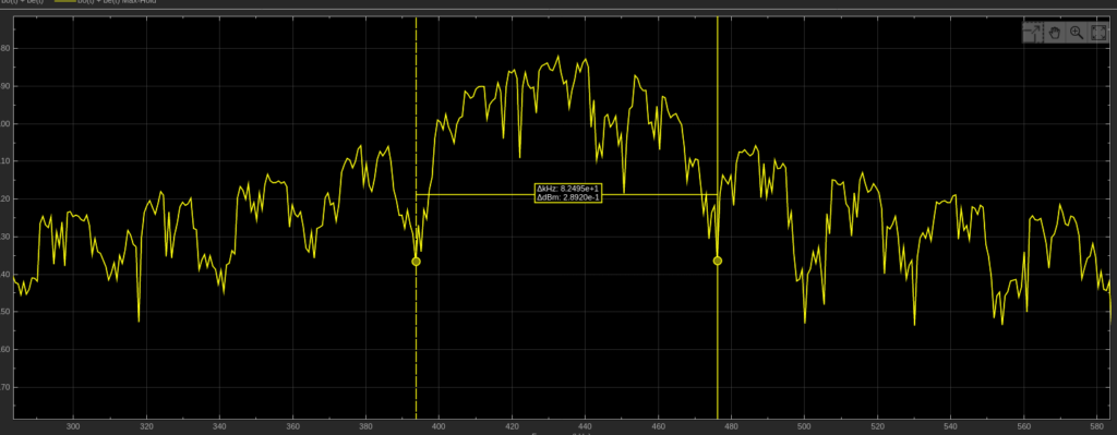
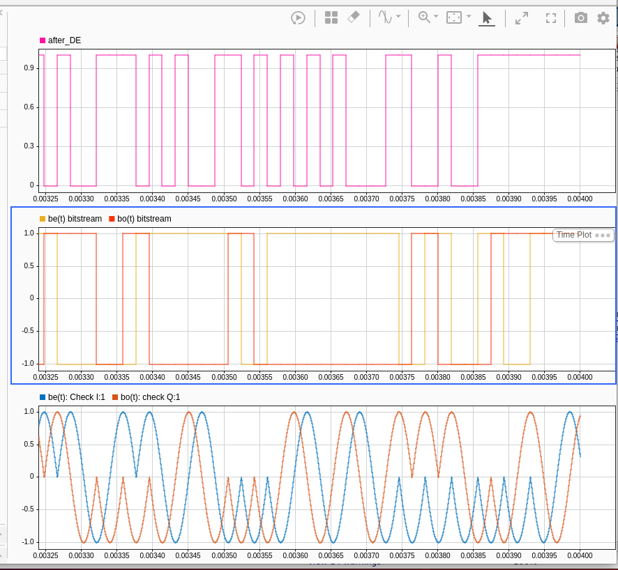
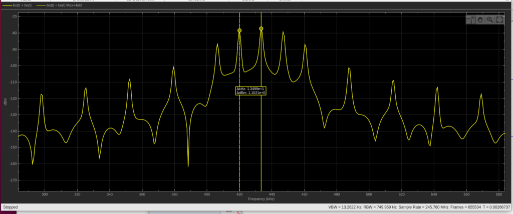
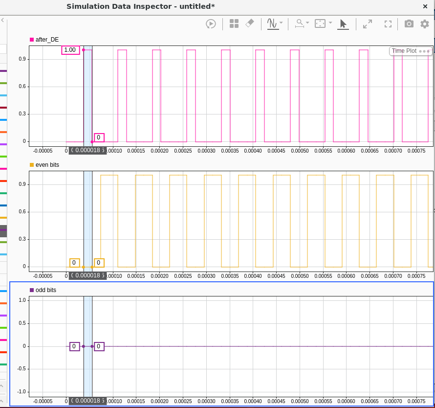
Finding Optimal Sync Words for Digital Voice Protocols
A Day at Dwingeloo
Comment and Critique on “Real and Complex Signal Basics” Article in QEX September/October 2025
Response to Pete’s Technical Critique
Hi Pete,
Thank you so much for taking the time to provide such detailed technical feedback! I really appreciate your careful reading. You’ve raised some important points that deserve thoughtful responses. Let me try and address each one.
Filtering Out the Lower Image and Complex-Valued Signals
I was imprecise here. My statement “Let’s filter out the lower image, and transmit fc” could be misleading in the context I presented it.
What I was trying to convey to a general audience is the conceptual process that happens in single-sideband modulation when we move to complex baseband representation. What you are saying is that by placing this immediately after showing Euler’s identity for a real cosine, I created confusion about what’s actually transmittable.
You’re correct that if we literally kept only the positive frequency component (α/2)e^(i2πfct), we’d have a complex-valued signal that cannot be transmitted with a single real antenna. In the article’s pedagogical flow, I should have either
1. Been more explicit that this is a conceptual stepping stone to understanding quadrature modulation, or
2. Maintained the real signal throughout this section and introduced the complex representation only when discussing I/Q modulation
Your point is well-taken, and this section could be clarified for technical accuracy.
Sign Convention: I·cos(2πfct) + Q·sin(2πfct) vs. I·cos(2πfct) – Q·sin(2πfct)
This is a really interesting point about convention. You’re right that most DSP textbooks use the negative sign on the sinusoid: I·cos(2πfct) – Q·sin(2πfct), and you’ve identified the key reason. It is consistency with Fourier transform conventions and phase modulation.
For the article’s target audience (QEX readers who are typically radio amateurs with varying levels of DSP background), I made a deliberate choice to use the positive sinusoid form because it’s simpler to explain without being technically wrong.
The positive form I·cos + Q·sin maps more directly to the “cosine on I-axis, sine on Q-axis” geometric intuition that I was building. There is also a hardware convention. The RF engineering texts and datasheets that I have used for I/Q modulators use the positive convention much more often than negative. For readers less comfortable with complex notation, introducing the negative sign requires explaining that it ultimately comes from the complex number properties. This has been a turn-off for people in the past. I did not want it to be a turn off for QEX.
That said, you’re absolutely correct that the negative convention gives cos(2πfct + θ) for phase modulation (standard trig identity). The positive convention gives cos(2πfct – θ), which is non-standard. For frequency modulation, the derivative relationship works correctly only with the negative convention. The negative form aligns with Re{(I + iQ)e^(i2πfct)}
In retrospect I could have used the standard negative convention from the start, or explicitly acknowledged the existence of both conventions and explained why I chose one over the other. Since this is the identical treatment that I got from my grad school notes, I’m not the only person to explain it this way. It is, however, a compromise.
Integration of Cosine from 0 to T Being Zero
This is a significant oversimplification on my part. You’re absolutely right that ∫₀^Tsym cos(2π(2fc)t)dt = sin(2π(2fc)Tsym)/(4πfc), which is generally not zero.
What I meant to convey (but obviously failed to state clearly) is that when we integrate cos(2π(2fc)t) over many symbol periods, or when the symbol period Tsym is chosen to be an integer multiple of the carrier period, the integral approaches zero. In practical systems, the low-pass filter following the mixer rejects the 2fc components.
I should have written something like: “We use a low-pass filter to remove the 2fc terms, leaving us with the DC component from the integration” rather than claiming the integral itself is zero.
This is an important distinction, especially for readers who might try to work through the math themselves. The pedagogical shortcut I took could definitely cause confusion when students try to verify the math or understand DTFT/FFT concepts later. Thank you for the reference to Figure 3-2 in your textbook (which I have). I am sure that many people will take a look.
Image Elimination
You’ve identified another important imprecision. When I wrote “we eliminate an entire image,” I was trying to express that quadrature modulation produces a single-sideband spectrum rather than the double-sideband spectrum of a real carrier. I wanted to stop there because this is something useful in practical radio designs.
Your math clearly shows that the real carrier: I·cos(2πfct) produces symmetric images at ±fc and the quadrature: I·cos(2πfct) + Q·sin(2πfct) = (I/2 + Q/2i)e^(i2πfct) + (I/2 – Q/2i)e^(-i2πfct)
You’re right that this doesn’t automatically or magically eliminate an image. Both positive and negative frequency components exist. However, the key advantage is that with independent control of I and Q, we can create single-sideband modulation where the negative frequency component can be zeroed out.
I should have been more precise: quadrature modulation *enables* single-sideband transmission through appropriate choice of I and Q, rather than automatically eliminating an image.
Feedback like this highlights the challenge of writing about DSP for a mixed audience. Trying to build intuition without sacrificing technical accuracy. I absolutely favor paths towards intuitive explanation I absolutely can and do create technical errors in the process. Being more rigorous with the mathematics, and/or explicitlly noting where there’s a simplication, is something I will take to heart in any future submissions.
I really appreciate you taking the time to work through these details. Our tradition at ORI is to welcome comment and critique. Thank you!
-Michelle Thompson
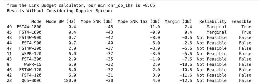
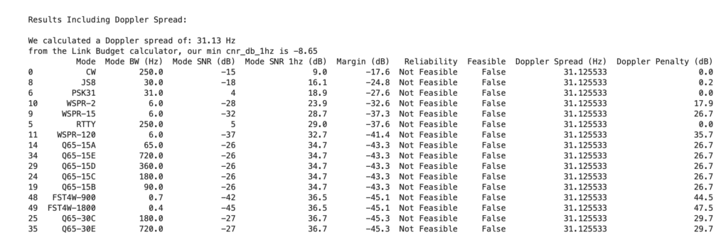
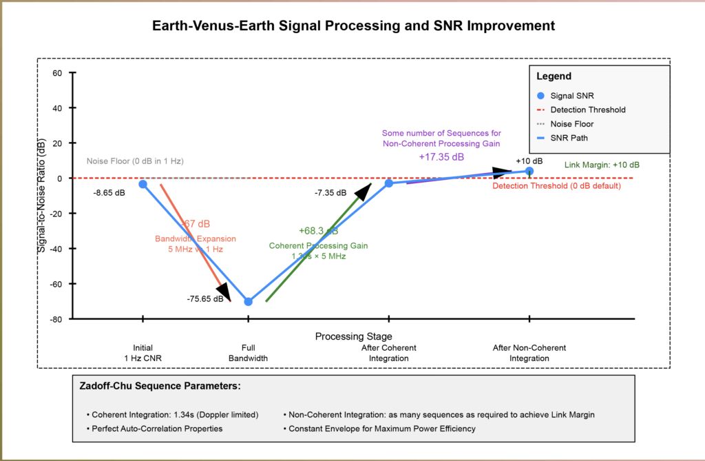
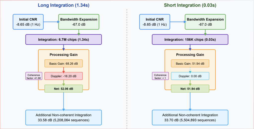
FunCube+ Mode Dynamic Transponder Analysis and Simulation Model for AMSAT-UK
Inner Circle Sphere of Activity
If you know of an event that would welcome ORI, please let your favorite board member know at our hello at openresearch dot institute email address.
1 September 2025 Our Complex Modulation Math article was published in ARRL’s QEX magazine in the September/October issue. See this issue for a comment and critique, and response!
5 September 2025 – Charter for the current Technological Advisory Council of the US Federal Communications Commission concluded.
19-21 September 2025 – ESA and AMSAT-DLworkshop was held in Bochum, Germany.
3 October 2025 – Deadline for submission for FCC TAC membership was met. Two volunteers applied for membership in the next available TAC.
10-12 October 2025 – Presentation given at Pacificon, San Ramon Marriot, CA, USA. Recording available on our YouTube channel.
11-12 October 2025– Presentation given to AMSAT-UK Symposium, and collaboration with AMSAT-UK commenced. See this issue for more details about MDT.
Thank you to all who support our work! We certainly couldn’t do it without you.
Anshul Makkar, Director ORI
Keith Wheeler, Secretary ORI
Steve Conklin, CFO ORI
Michelle Thompson, CEO ORI
Matthew Wishek, Director ORI